This post is part of the SATF work.

Ideas from the “Solution” and “Probabilistic testing” sections applied to the reality and devices of the MRDS framework gave birth to the simulation acceptance test execution procedure depicted on the picture below. Every step of it will be illustrated by the Monte Carlo localization test of the “Test example” section.

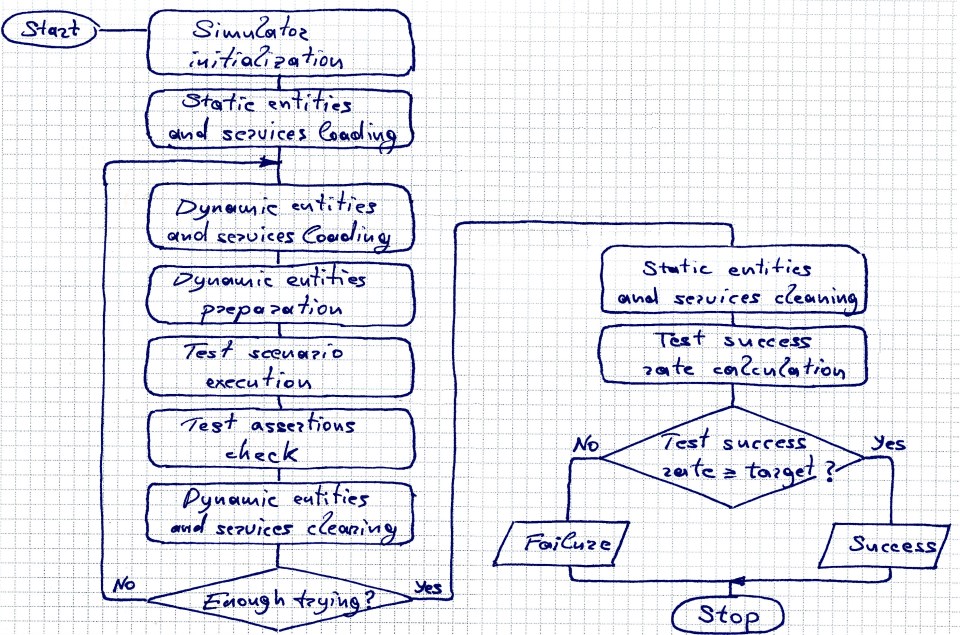Simulation acceptance test execution procedure

On the very first step, the simulation test runner sets up the simulator engine according to the test’s preferences – for now, it amounts to tuning of the physics simulation quality. In the example, the vehicle itself is quite primitive, and almost no physical interaction is expected, so the test contents with the lowest physics simulation quality.

Then the test runner loads static objects – simulation entities and services, whose state is not going to change through the test run. As such, they don’t have to be reloaded on each test try. This object’s division into static and dynamic becomes important in the context of the test runner implementation, because the entity load and service launch operations are expensive, and their number should be minimized. In the example, the number of static physics primitives comprising the building walls and the floor is 24 versus 35 in total. On the contrary, only 1 of 6 services in total is static – the MapProvider service, providing the fixed map of the building.

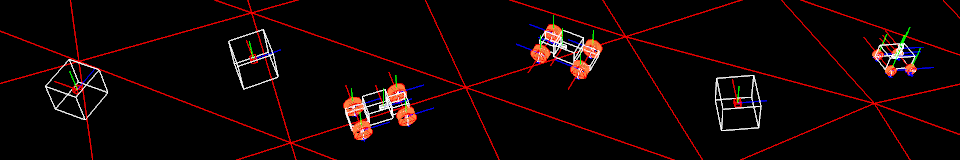
At that point, the static part of the test is prepared, and the dynamic phase starts. The test runner loads dynamic entities and launches dynamic services, those things that change their state during the test execution. In the localization example, dynamic are the robot entity, moving over the test run, and the localization service, tracking its position. All entities’ and services’ initial state is taken from corresponding files. But the tests have an option to alter the state of the newly loaded dynamic entities, perhaps, to introduce some random noise like in the cross country example from the “Probabilistic testing” section.

Now everything is loaded, and the test try is ready for execution. The test runner commences the test scenario. In the global localization with curved trajectory example test, it consists of move straight, wait, turn right, wait, move straight, wait, and stop commands. When the test try is over, the test runner checks the test’s assertions, in example case, comparing the pose from MC localization service with the robot’s pose acquired from the physics simulation. Then the test runner logs the result and proceeds to fixture cleaning. At that point, cleaning concerns only dynamic objects: dynamic simulation entities are removed from the simulated environment, dynamic services are dropped. And control returns to the beginning of dynamic phase, starting the next test try.

When all test tries are exhausted, the test finishes: the test runner drops down remaining static services and entities, calculates the test’s resultant success rate, compares it with the test target and, at last, declares a success or failure. Now, the test runner is ready for the next auto acceptance simulation test…